Optimization Algorithms for Cost Functions
*note* The reception has been great! Please leave a comment to let me know what I should tackle next
An objective function is a function one is trying to minimize with respect to a set of parameters. In machine learning, the objective function is often set to a measure of how similar a predicted value is to the actual value. Usually, we are looking to find the set of parameters that lead to the smallest possible cost which would imply that your algorithm will perform well. The smallest cost possible of a function is known as the minima. Sometimes a cost function can have multiple local minima. Fortunately, with very high dimensional parameter spaces, local minima that prevent sufficient optimization of the objective function do not occur very often because it would imply that every parameter is concave at the same time early in the process. This is typically not the case, and so we are left with a lot of saddles instead of true minima.


Algorithms that find the set of parameters that lead to the minima are known as optimization algorithms. As the algorithms increase in complexity, we’ll see that they tend to try to get to the minima more efficiently. The one’s we’ll discuss in this post include:
- Stochastic Gradient Descent
- Momentum
- RMSProp
- The Adam Algorithms
Stochastic Gradient Descent
If you’ve seen my “Logistic Regression Made Easy” post then we’ve already seen an example of how stochastic gradient descent works. If you look up Stochastic Gradient Descent (SGD) you will most likely come across an equation that looks like this:

They’ll tell you that theta is the parameter you’re trying to find the optimum value that minimizes J. J here is referred to as the objective function. Finally we have the learning rate which is labeled as alpha. They’ll tell you to repeatedly evaluate this function until you reach the desired cost.
What does it mean? Think for a second that you’re sitting on sled at the top of one hill, looking out towards another hill. If you slide down the hill, you will naturally move down it until you eventually come to a rest at the bottom. If the first hill is steep enough, you might start going up the side of the next hill. In this analogy you can think of:
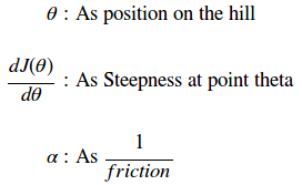
A high learning rate would imply low friction and therefore the sled would zoom along the hill as if on ice. A low learning rate would imply high friction, and so the sled would struggle to move down the hill as if on carpet. How do we simulate this effect with something like the equation above?
Stochastic Gradient Descent
- Initialize parameters (thetas, learning rate)
- Compute the gradient at each theta
- Update Parameters
- Repeat steps 2 and 3 until cost stabilizes
Lets come up with a simple example to see how this works!
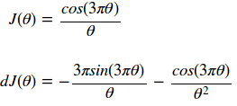
here we see an objective function and its derivative (gradient):
we can generate a plot of the function and 1/30th its gradient with the code below
import numpy as np

def minimaFunction(theta):
return np.cos(3*np.pi*theta)/theta

def minimaFunctionDerivative(theta):
const1 = 3*np.pi
const2 = const1*theta
return -(const1*np.sin(const2)/theta)-np.cos(const2)/theta**2

theta = np.arange(.1,2.1,.01)
Jtheta = minimaFunction(theta)
dJtheta = minimaFunctionDerivative(theta)

plt.plot(theta,Jtheta,label = r'$J(\theta)$')
plt.plot(theta,dJtheta/30,label = r'$dJ(\theta)/30$')
plt.legend()
axes = plt.gca()
#axes.set_ylim([-10,10])

plt.ylabel(r'$J(\theta),dJ(\theta)/30$')
plt.xlabel(r'$\theta$')
plt.title(r'$J(\theta),dJ(\theta)/30 $ vs $\theta$')
plt.show()

Two things stand out in the plot above. First, notice how this cost function has a few minima (around .25,1.0, and 1.7). Second, notice how the derivative is equal to zero at the minima and large at the inflection points. This characteristic is what we will take advantage of in SGD.
We can see an implementation of the four steps above in the following code. It will also generate a video that shows the value of theta and and the gradient at each step.
import numpy as np
import matplotlib.pyplot as plt
import matplotlib.animation as animation

def optimize(iterations, oF, dOF,params,learningRate):
"""
computes the optimal value of params for a given objective function and its derivative
Arguments:
- iteratoins - the number of iterations required to optimize the objective function
- oF - the objective function
- dOF - the derivative function of the objective function
- params - the parameters of the function to optimize
- learningRate - the learning rate
Return:
- oParams - the list of optimized parameters at each step of iteration
"""
oParams = [params]
#The iteration loop
for i in range(iterations):
# Compute the derivative of the parameters
dParams = dOF(params)
# Compute the update
params = params-learningRate*dParams

# app end the new parameters
oParams.append(params)

return np.array(oParams)

def minimaFunction(theta):
return np.cos(3*np.pi*theta)/theta

def minimaFunctionDerivative(theta):
const1 = 3*np.pi
const2 = const1*theta
return -(const1*np.sin(const2)/theta)-np.cos(const2)/theta**2

theta = .6
iterations=45
learningRate = .0007
optimizedParameters = optimize(iterations,\
minimaFunction,\
minimaFunctionDerivative,\
theta,\
learningRate)
That seems to work pretty well! You should notice that if the initial value of theta is larger, the optimization algorithm will wind up in one of the other local minima. However, as mentioned above, the chance of a poorly, performing, true minima existing in an extremely high dimensional space is unlikely because it would require all parameters to be concave at the same time.
You might wonder, “What happens if our learning rate is too large?”. If the step size is too large, then the algorithm might never find the optimal as seen in the animation below. Its important to monitor the cost function and make sure that it is generally monotonically decreasing. If its not, you may find that you have to decrease the learning rate.
SGD also works in the case of multi variate parameter spaces. We can plot a 2D function as a contour plot. Here you can see the SGD work on an asymmetric bowl function.
import numpy as np
import matplotlib.mlab as mlab
import matplotlib.pyplot as plt
import scipy.stats
import matplotlib.animation as animation

def minimaFunction(params):
#Bivariate Normal function
X,Y = params

sigma11,sigma12,mu11,mu12 = (3.0,.5,0.0,0.0)

Z1 = mlab.bivariate_normal(X, Y, sigma11,sigma12,mu11,mu12)

Z = Z1

return -40*Z

def minimaFunctionDerivative(params):
# Derivative of the bivariate normal function
X,Y = params

sigma11,sigma12,mu11,mu12 = (3.0,.5,0.0,0.0)

dZ1X = -scipy.stats.norm.pdf(X, mu11, sigma11)*(mu11 - X)/sigma11**2
dZ1Y = -scipy.stats.norm.pdf(Y, mu12, sigma12)*(mu12 - Y)/sigma12**2

return (dZ1X,dZ1Y)

def optimize(iterations, oF, dOF,params,learningRate,beta):
"""
computes the optimal value of params for a given objective function and its derivative
Arguments:
- iteratoins - the number of iterations required to optimize the objective function
- oF - the objective function
- dOF - the derivative function of the objective function
- params - the parameters of the function to optimize
- learningRate - the learning rate
- beta - The weighted moving average parameter
Return:
- oParams - the list of optimized parameters at each step of iteration
"""
oParams = [params]
vdw     = (0.0,0.0)
#The iteration loop
for i in range(iterations):
# Compute the derivative of the parameters
dParams = dOF(params)

#SGD in this line Goes through each parameter and applies parameter = parameter -learningrate*dParameter
params = tuple([par-learningRate*dPar for dPar,par in zip(dParams,params)])

# append the new parameters
oParams.append(params)

return oParams

iterations=100
learningRate = 1
beta = .9
x,y = 4.0,1.0
params = (x,y)
optimizedParameters = optimize(iterations,\
minimaFunction,\
minimaFunctionDerivative,\
params,\
learningRate,\
beta)
SGD With Momentum
There is one caveat that traditional SGD does not address. Typically, users want to use very large learning rates to quickly learn the parameters of interest. Unfortunately, when the cost surface is narrow, this can lead to instability. You can see that in the form of the thrashing in the y parameter direction in the previous video coupled with the lack of horizontal progress towards the minima. Momentum attempts to address this problem by making predictions that are informed by past gradients. Typically, SGD with Momentum updates parameters with the following equation:

The gamma and nu values allow the user to weight the previous and current value of dJ(theta) to determine the new value of theta. It is pretty common for people to select values for gamma and nu to create an exponential weighted moving average as follows:
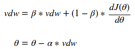
A good starting point for the beta parameter is 0.9. Selecting a value of beta equal to 1-1/t allows the user to more strongly consider the last t values of vdw. This simple change in the optimization can create dramatic results! We can now use a much larger learning rate and converge on the solution in a fraction of the time!
import numpy as np
import matplotlib.mlab as mlab
import matplotlib.pyplot as plt
import scipy.stats
import matplotlib.animation as animation

def minimaFunction(params):
#Bivariate Normal function
X,Y = params

sigma11,sigma12,mu11,mu12 = (3.0,.5,0.0,0.0)

Z1 = mlab.bivariate_normal(X, Y, sigma11,sigma12,mu11,mu12)

Z = Z1

return -40*Z

def minimaFunctionDerivative(params):
# Derivative of the bivariate normal function
X,Y = params

sigma11,sigma12,mu11,mu12 = (3.0,.5,0.0,0.0)

dZ1X = -scipy.stats.norm.pdf(X, mu11, sigma11)*(mu11 - X)/sigma11**2
dZ1Y = -scipy.stats.norm.pdf(Y, mu12, sigma12)*(mu12 - Y)/sigma12**2

return (dZ1X,dZ1Y)

def optimize(iterations, oF, dOF,params,learningRate,beta):
"""
computes the optimal value of params for a given objective function and its derivative
Arguments:
- iteratoins - the number of iterations required to optimize the objective function
- oF - the objective function
- dOF - the derivative function of the objective function
- params - the parameters of the function to optimize
- learningRate - the learning rate
- beta - The weighted moving average parameter for momentum
Return:
- oParams - the list of optimized parameters at each step of iteration
"""
oParams = [params]
vdw     = (0.0,0.0)
#The iteration loop
for i in range(iterations):
# Compute the derivative of the parameters
dParams = dOF(params)

# Compute the momentum of each gradient vdw = vdw*beta+(1.0+beta)*dPar
vdw = tuple([vDW*beta+(1.0-beta)*dPar for dPar,vDW in zip(dParams,vdw)])

#SGD in this line Goes through each parameter and applies parameter = parameter -learningrate*dParameter
params = tuple([par-learningRate*dPar for dPar,par in zip(vdw,params)])

# append the new parameters
oParams.append(params)

return oParams

iterations=100
learningRate = 5.3
beta = .9
x,y = 4.0,1.0
params = (x,y)
optimizedParameters = optimize(iterations,\
minimaFunction,\
minimaFunctionDerivative,\
params,\
learningRate,\
beta)
RMSProp
Like everything in engineering, we’re always striving to do better. RMS prop tries to improve on the momentum function by observing that the gradient of the function with respect to each parameter will be relatively large or small to one another. Because of this, we are able take a weighted exponential moving average of the square of each gradient and normalize the gradient descent function proportionally. Parameters with large gradients will become much larger than parameters with small gradients and allow a smooth descent to the optimal value. This can be seen in the following equation:
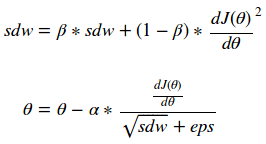
Note that the epsilon here is added for numerical stability and can take on values of 10e-7. What does this look like?
import numpy as np
import matplotlib.mlab as mlab
import matplotlib.pyplot as plt
import scipy.stats
import matplotlib.animation as animation

def minimaFunction(params):
#Bivariate Normal function
X,Y = params

sigma11,sigma12,mu11,mu12 = (3.0,.5,0.0,0.0)

Z1 = mlab.bivariate_normal(X, Y, sigma11,sigma12,mu11,mu12)

Z = Z1

return -40*Z

def minimaFunctionDerivative(params):
# Derivative of the bivariate normal function
X,Y = params

sigma11,sigma12,mu11,mu12 = (3.0,.5,0.0,0.0)

dZ1X = -scipy.stats.norm.pdf(X, mu11, sigma11)*(mu11 - X)/sigma11**2
dZ1Y = -scipy.stats.norm.pdf(Y, mu12, sigma12)*(mu12 - Y)/sigma12**2

return (dZ1X,dZ1Y)

def optimize(iterations, oF, dOF,params,learningRate,beta):
"""
computes the optimal value of params for a given objective function and its derivative
Arguments:
- iteratoins - the number of iterations required to optimize the objective function
- oF - the objective function
- dOF - the derivative function of the objective function
- params - the parameters of the function to optimize
- learningRate - the learning rate
- beta - The weighted moving average parameter for RMSProp
Return:
- oParams - the list of optimized parameters at each step of iteration
"""
oParams = [params]
sdw     = (0.0,0.0)
eps = 10**(-7)
#The iteration loop
for i in range(iterations):
# Compute the derivative of the parameters
dParams = dOF(params)

# Compute the momentum of each gradient sdw = sdw*beta+(1.0+beta)*dPar^2
sdw = tuple([sDW*beta+(1.0-beta)*dPar**2 for dPar,sDW in zip(dParams,sdw)])

#SGD in this line Goes through each parameter and applies parameter = parameter -learningrate*dParameter
params = tuple([par-learningRate*dPar/((sDW**.5)+eps) for sDW,par,dPar in zip(sdw,params,dParams)])

# append the new parameters
oParams.append(params)

return oParams

iterations=10
learningRate = .3
beta = .9
x,y = 5.0,1.0
params = (x,y)
optimizedParameters = optimize(iterations,\
minimaFunction,\
minimaFunctionDerivative,\
params,\
learningRate,\
beta)
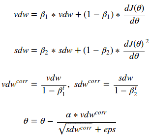
The Adam Algorithm
The Adam Algorithm combines the notions of momentum and RMSProp into one algorithm to get the best of both worlds. Its formulation can be seen below as:
import numpy as np
import matplotlib.mlab as mlab
import matplotlib.pyplot as plt
import scipy.stats
import matplotlib.animation as animation

def minimaFunction(params):
#Bivariate Normal function
X,Y = params

sigma11,sigma12,mu11,mu12 = (3.0,.5,0.0,0.0)

Z1 = mlab.bivariate_normal(X, Y, sigma11,sigma12,mu11,mu12)

Z = Z1

return -40*Z

def minimaFunctionDerivative(params):
# Derivative of the bivariate normal function
X,Y = params

sigma11,sigma12,mu11,mu12 = (3.0,.5,0.0,0.0)

dZ1X = -scipy.stats.norm.pdf(X, mu11, sigma11)*(mu11 - X)/sigma11**2
dZ1Y = -scipy.stats.norm.pdf(Y, mu12, sigma12)*(mu12 - Y)/sigma12**2

return (dZ1X,dZ1Y)

def optimize(iterations, oF, dOF,params,learningRate,beta1,beta2):
"""
computes the optimal value of params for a given objective function and its derivative
Arguments:
- iteratoins - the number of iterations required to optimize the objective function
- oF - the objective function
- dOF - the derivative function of the objective function
- params - the parameters of the function to optimize
- learningRate - the learning rate
- beta1 - The weighted moving average parameter for momentum component of ADAM
- beta2 - The weighted moving average parameter for RMSProp component of ADAM
Return:
- oParams - the list of optimized parameters at each step of iteration
"""
oParams = [params]
vdw     = (0.0,0.0)
sdw     = (0.0,0.0)
vdwCorr = (0.0,0.0)
sdwCorr = (0.0,0.0)

eps = 10**(-7)
#The iteration loop
for i in range(iterations):
# Compute the derivative of the parameters
dParams = dOF(params)

# Compute the momentum of each gradient vdw = vdw*beta+(1.0+beta)*dPar
vdw     = tuple([vDW*beta1+(1.0-beta1)*dPar for dPar,vDW in zip(dParams,vdw)])

# Compute the rms of each gradient sdw = sdw*beta+(1.0+beta)*dPar^2
sdw     = tuple([sDW*beta2+(1.0-beta2)*dPar**2.0 for dPar,sDW in zip(dParams,sdw)])
# Compute the weight boosting for sdw and vdw
vdwCorr = tuple([vDW/(1.0-beta1**(i+1.0)) for vDW in vdw])
sdwCorr = tuple([sDW/(1.0-beta2**(i+1.0)) for sDW in sdw])

#SGD in this line Goes through each parameter and applies parameter = parameter -learningrate*dParameter
params = tuple([par-learningRate*vdwCORR/((sdwCORR**.5)+eps) for sdwCORR,vdwCORR,par in zip(vdwCorr,sdwCorr,params)])

# append the new parameters
oParams.append(params)

return oParams

iterations=100
learningRate = .1
beta1 = .9
beta2 = .999
x,y = 5.0,1.0
params = (x,y)
optimizedParameters = optimize(iterations,\
minimaFunction,\
minimaFunctionDerivative,\
params,\
learningRate,\
beta1,\
beta2)</div>
The Adam algorithm is probably the most widely used optimization algorithm in Deep Learning these days. It seems to work well in a variety of applications and is my “go to” algorithm. You will notice that Adam computes a vdwcorr value. That value is used to “warm up” the exponentially weighted moving average. It will normalized the values by boosting them inversely proportional to the number of iterations that have passed. There are some good initial values to try when using Adam. Its probably best to start with a beta1 of .9 and a beta2 of .999.
Conclusions
There are quite a few choices when picking how to optimize your input parameters as a function of the objective function. In the above example we found that convergence for each method became faster and faster:
– SGD: 100 iterations
– SGD+Momentum: 50 Iterations
– RMSProp: 10 Iterations
– ADAM: 5 Iterations
Now you have some tools to take out into the real world! Have fun! As usual you can find my full jupyter notebook and source code on my Github

Wow, this is absolutely amazing. I kept trying to understand it but couldn’t they usually don’t have any coding examples. Thank you very much for the post.
LikeLike
Thanks Raza! I’m trying to take my time and think about what it was like for me to learn for the first time as well. I’m thinking about my next post now, do you have any suggestions or recommendations?
LikeLike
It’s great to come across a blog every once in a while that isn’t the same out of date rehashed material. Fantastic read.
LikeLike